This blog goes through a simple linear regression that has an interaction between two variables. It will explain how you interpret the results and how to make some nice and simple figures.
I found this other great blog that would also be worth checking out, this is going to be pretty similar to it!
https://biologyforfun.wordpress.com/2014/04/08/interpreting-interaction-coefficient-in-r-part1-lm/
Anyway, step 1 is to make up some data. Note: this is some code that will work in r.
I found this other great blog that would also be worth checking out, this is going to be pretty similar to it!
https://biologyforfun.wordpress.com/2014/04/08/interpreting-interaction-coefficient-in-r-part1-lm/
Anyway, step 1 is to make up some data. Note: this is some code that will work in r.
#Simulate some data
# Get two covariates, each with 100 observations.
Data<-data.frame(humid = rnorm(100,30,0.5), temperature = rnorm(100,25))
# simulate Y data. Note that the slope for X2 is set to 0.
mu <- 1 + 2 * Data$humid + 0 * Data$temperature #linear equation
Data$mass <- rnorm(100, mean = mu, sd = 0.5)
plot(mass~humid, Data)
plot(mass~temperature, Data)
#You want to centre your explanatory variables
Data$humid.cnt <- humid - mean(humid)
Data$temperature.cnt <- temperature - mean(temperature)
model<- lm(mass ~ humid.cnt + temperature.cnt + humid*temperature, data=Data)
summary(model)
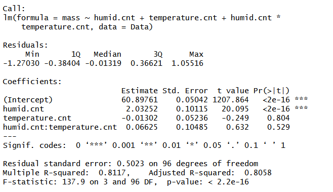
Output results explained
I’m just going to focus on the coefficients in this blog. This is how you interpret the estimates. First, the estimate for the intercept (60.89) is the mean mass as average humidity and temperature. If you did not centre humidity and temperature, it would tell you the mean mass when humidity and temperature were 0, which is not very useful because that never happens! This is almost always the case with biological data! The humid.cnt estimate (2.03252) tells you that with an increase in 1 unit of humidity, mass will increase by about 2 grams (i.e. this is the slope of mass over humidity) for mean temperature. The temperature.cnt estimate (-0.01302) tells you that with an increase in 1°C, mass will decrease by 0.01302 grams (i.e. this is the slope of mass over temperature) for mean humidity. The last one is the interaction term, humid.cnt:temperature.cnt, and this is saying that, although humidity increases mass by 2.03252 grams per unit at the mean temperature, if temperature was actually 1°C above the mean, then the effect of humidity on mass would change to 2.0195 (2.03252 + -0.01302).
If temperatures were 10°C warmer than average, then the slope of mass over humidity would be 1.9 (2.03252 + (-0.01302*10)).
If temperatures were 5°C colder than average, then the slope of mass over humidity would be 2.10 (2.03252 + (-0.01302*-5)).
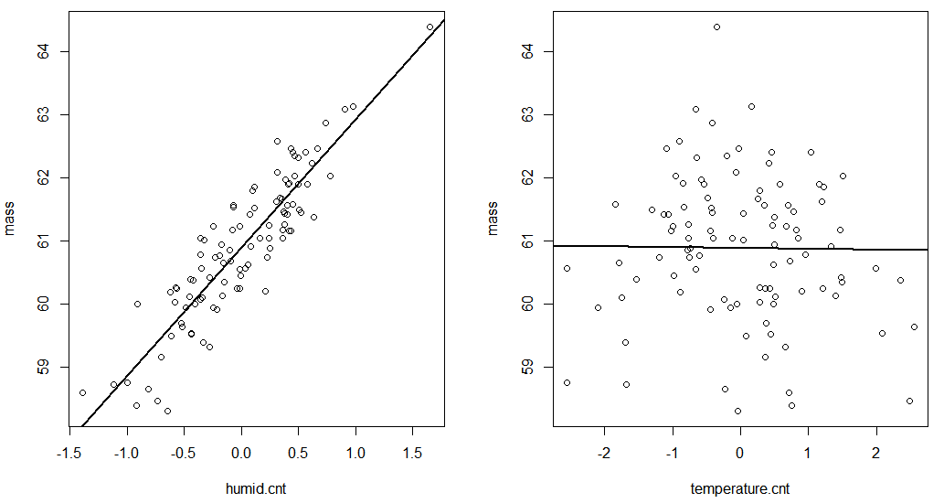
Plots
Ok, let’s start out easy and plot the single effect of humidity on mass, and then temperature on mass.
I’m just going to focus on the coefficients in this blog. This is how you interpret the estimates. First, the estimate for the intercept (60.89) is the mean mass as average humidity and temperature. If you did not centre humidity and temperature, it would tell you the mean mass when humidity and temperature were 0, which is not very useful because that never happens! This is almost always the case with biological data! The humid.cnt estimate (2.03252) tells you that with an increase in 1 unit of humidity, mass will increase by about 2 grams (i.e. this is the slope of mass over humidity) for mean temperature. The temperature.cnt estimate (-0.01302) tells you that with an increase in 1°C, mass will decrease by 0.01302 grams (i.e. this is the slope of mass over temperature) for mean humidity. The last one is the interaction term, humid.cnt:temperature.cnt, and this is saying that, although humidity increases mass by 2.03252 grams per unit at the mean temperature, if temperature was actually 1°C above the mean, then the effect of humidity on mass would change to 2.0195 (2.03252 + -0.01302).
If temperatures were 10°C warmer than average, then the slope of mass over humidity would be 1.9 (2.03252 + (-0.01302*10)).
If temperatures were 5°C colder than average, then the slope of mass over humidity would be 2.10 (2.03252 + (-0.01302*-5)).
Plots
Ok, let’s start out easy and plot the single effect of humidity on mass, and then temperature on mass.
#Run the model
model<- lm(mass ~ humid.cnt + temperature.cnt + humid.cnt*temperature.cnt, data=Data)
summary(model)
#Let's create a new data frame with the coefficients in them
coef <- data.frame(summary(model)$coefficients)
#Make a new column from row names that we can use
coef$variables<-row.names(coef)
#Get the intercept and slope values
int<- coef$Estimate[coef$variables=="(Intercept)"]
slope.humid<- coef$Estimate[coef$variables=="humid.cnt"]
slope.temperature <- coef$Estimate[coef$variables=="temperature.cnt"]
interaction <- coef$Estimate[coef$variables=="humid.cnt:temperature.cnt"]
#Lets try plotting
par(mfrow=c(1,2)) #Plot next to each other
#1. Mass ~ Humidity
plot(mass~humid.cnt, Data)
abline(int, slope.humid, lwd=2) #the effect of humidity on mass for mean temperature
#2. Mass ~ Temperature
plot(mass~temperature.cnt, Data)
abline(int, slope.temperature, lwd=2)
dev.off()
The two plots should look like this:
Now lets try and plot the interaction. Ideally, this would be a 3d plot where you could see how mass changed with changes in humidity and temperature simultaneously. But often we aren’t interested in that level of information. Say we are more interested in understanding the effects of humidity, but want to know how they change with different temperatures, this is an easy option. Note: the legend look code messy because without adding the function formattable you end up with really long temperature values (around 10 decimal places which looks terrible).
#3. Mass ~ Humidity but add the information about how this changes with temperature
#Look at the 1st and 3rd quantiles (rather than min and max temperatures which occur much less frequently in real life)
quantiles <- quantile((Data$temperature.cnt), c(0.25, 0.75))
#Plot Mass ~ Humidity
plot(mass ~ humid.cnt, Data)
abline(int, slope.humid, lwd=2)
#Add the slopes for the hotter and colder temperatures
abline( int , slope + (interaction * quantiles[[1]]),col="blue", lwd=2) #Cooler temperatures
abline( int , slope + (interaction * quantiles[[2]]),col="red", lwd=2) #Hotter temperatures
legend(min(Data$humid.cnt),max(Data$mass), c(paste("Mean", formattable(mean.Temp, digits=3), "Temperature"),paste(formattable((quantiles[[2]]+mean.Temp),digits=3), "Temperature"),paste(formattable((quantiles[[1]]+mean.Temp),digits=3), "Temperature")),lty=1,col=c("black" ,"red","blue"),bty="n",lwd=2)
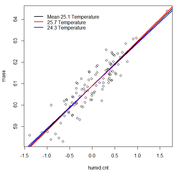
The plot suggests there is not a very large difference in how mass responds to humidity at different temperatures.
Too lazy to do this all yourself? Try this function!
This function will plot it for you! So now you don’t need to do any of the above, just run the function copied below and then type in:
plotInteraction(model,Data)
plotInteraction(model,Data)
plotInteraction <- function(model,Data){
#Let's create a new data frame with the coefficients in them
coef <- data.frame(summary(model)$coefficients)
#Make a new column from row names that we can use
coef$variables<-row.names(coef)
#Find the variables that are in the interaction term
for(i in 1:nrow(coef)){
if(length(grep(":", coef$variables[i]))==1){
row <- i
}
}
vars <- strsplit(coef$variables[row], ":")
var1 <- vars[[1]][1]
var2 <- vars[[1]][2]
response <- as.character(model$call[[2]][[2]])
#Get the intercept and slope values
int<- coef$Estimate[coef$variables=="(Intercept)"]
slope.1<- coef$Estimate[coef$variables == var1]
slope.2 <- coef$Estimate[coef$variables==var2]
interaction <- coef$Estimate[coef$variables==coef$variables[row]]
#Look at the 1st and 3rd quantiles rather than min and max temperatures.
quantiles<-quantile(Data[,var2], c(0.25, 0.75))
#Plot Mass ~ Humidity
plot(Data[,response] ~ Data[,var1], Data, ylab=response, xlab= var1)
abline(int, slope.1, lwd=2)
#Add the slopes for the hotter and colder temperatures
abline( int , slope.1 + (interaction * quantiles[[1]]),col="blue", lwd=2) #Cooler temperatures
abline( int , slope.1 + (interaction * quantiles[[2]]),col="red", lwd=2) #Hotter temperatures
legend(min(Data[,var1]),max(Data[,response]), c(paste("Mean", var2),paste("Increase", formattable(quantiles[[2]],digits=4), var2),paste("Decrease", formattable((quantiles[[1]]),digits=3), var2)),lty=1,col=c("black" ,"red","blue"),bty="n",lwd=2)
}
 RSS Feed
